
Testing assumptions of one-sample t-test
Introduction
One sample t test is a parametric test that is used to determine whether a sample comes from a population with a specific mean not always known, but sometimes hypothesized. The hypothesized value, also known as test value may come from a trusted research organization, or industry standards.
For example, we may want to show that a new online teaching method for learners in Excel can improve their spreadsheet skills to the national average score. Our sample will be the test scores for learners who receive the new online teaching method in Excel, and the population mean is the national average test score.
Learning Outcomes
In this lesson, we’ll use a hypothetical data to illustrate how we can use SPSS to carry out one-sample t-test. By the time you complete the tutorial, you should be able to:
- check integrity of sample data ideal for one-sample t test
- test normality of sample data
- identify outliers in sample data
Problem Statement
According to an industrial standard, the average measurement of protein on each energy bar is 20 grams. In our study, we collect a random sample of 42 energy bars from a number of different stores to represent the population of energy bars available to the general consumer. We want to use one-sample t- test to confirm whether the labels on the bars claiming that each bar contains 20 grams of protein is indeed accurate. The weights of the 42 energy bars are shown in Table 1:
| 20.7 | 27.46 | 22.15 | 19.85 | 21.29 | 24.75 |
| 20.75 | 22.91 | 25.34 | 20.33 | 21.54 | 21.08 |
| 22.14 | 19.56 | 21.1 | 18.04 | 24.12 | 19.95 |
| 19.72 | 18.28 | 16.26 | 17.46 | 20.53 | 22.12 |
| 25.06 | 22.44 | 19.08 | 19.88 | 21.39 | 22.33 |
| 25.79 | 20.75 | 22.91 | 25.34 | 20.33 | 22.14 |
| 27.46 | 22.15 | 19.85 | 21.29 | 25.34 | 20.33 |
Data Requirements of Sample Data
The hypothetical data for our 42 energy bars must meet the following assumptions for the test on one-sample t-test to be valid:
Assumption 1: Random Sample
We can safely assume, from the given information that the collection of energy bars is a random sample from the population of energy bars available to the general consumer (i.e., a mix of lots of bars).
Assumption 2: Continuous Scale of Data
The test variable (energy bars) is measured on a continuous scale – in grams.
Assumption 3: Independent Datasets
The measurements of the 42 bars are independent. There is no relationship between weights in grams of the energy bars.
Assumption 4: Normal Distribution of Dataset
The data of 42 energy bars is approximately normally distributed as shown in the following example:
In the following illustration , we use SPSS procedures to show how to check the normality of our data by doing the following tasks:
1. Start SPSS
2. Create a dataset with the 42 energy bars
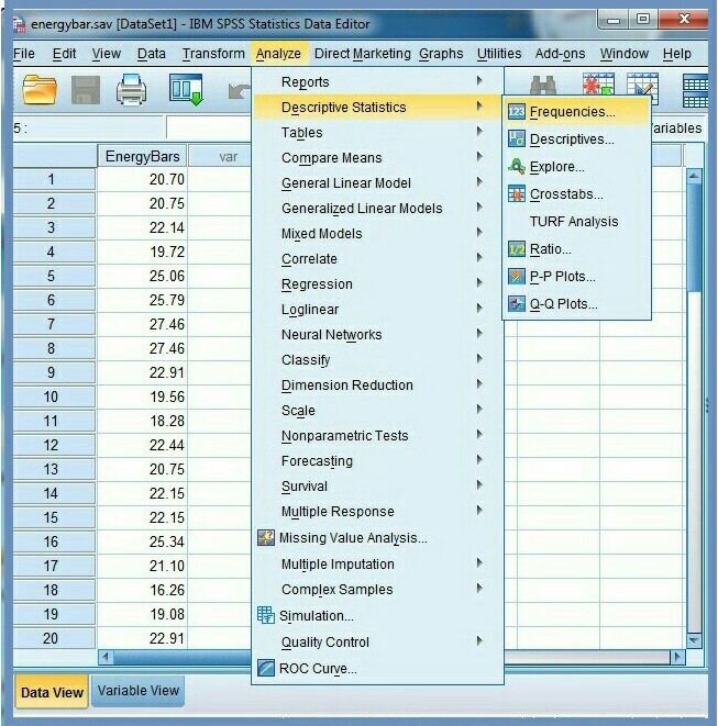
3. Click Analyze, Figure 1
4. Click Descriptive Statistics
5. Click Frequencies…
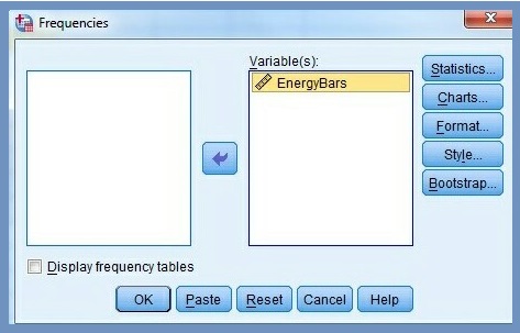
6. Select the test variable (energy bars) in the Frequencies dialog box, Figure 2.
7. Click the arrow button ![]() to move the variable to the test Variable(s) area. Figure 3 displays the test variable that has been moved to the test variable dialog box.
to move the variable to the test Variable(s) area. Figure 3 displays the test variable that has been moved to the test variable dialog box.
8. Click Display frequency tables checkbox to deselect it
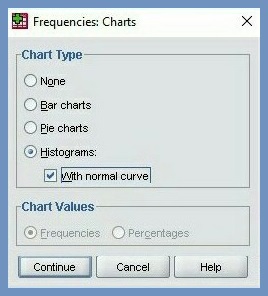
Our aim is to create a histogram. Therefore, we ignore all other commands and focus on Chart… command.
9. Click Chart… command
10. Select Histograms option in Frequencies Chart dialog box, Figure 4
11. Check Show normal curve on histogram, Figure 4
12. Click Continue
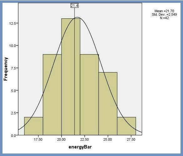
We now have a histogram, Figure 5. By inspection, the histogram shows the data curve is roughly bell-shaped, and symmetrical, which means they are “even” on both sides of the center. So, our assumption of a normal distribution of the energy bars data seems reasonable.
Assumption 5: Checking for Outliers
In a one-sample t-test, an important assumption is that there are no significant outliers in the data. Outliers can heavily skew results, as the t-test assumes that the sample data is approximately normally distributed. Figure 5 of the normality test and Table 1 shows no unusual patterns of data points within the 42 energy bars. By inspection, we can safely conclude that there are no significant outliers.
Citation Information
If you want to cite this lesson, you may use the following APA information:
- Author: Mahama, A.
- Date of publication: Use the 2023, February 27 or the last date the lesson was modified.
- Title: Conducting one sample t test
- URL of lesson: https://thecalleacademy.thecallinfo.com/course/data-analysis/lessons/conducting-one-sample-t-test/
- xxx is the date you retrieved the lesson from the online source
Example
Mahama, A. (2023, August 26). Conducting one sample t test. Retrieve xxx from https://thecalleacademy.thecallinfo.com/course/data-analysis/lessons/conducting-one-sample-t-test/
References
Daniel, T. (202017, December 10). One sample t test [Video]. Retrieved August 18, 2023 from https://www.youtube.com/watch?v=C2Qa5d9ij0Y
Editorial Director. (2023). How should p values be reported? Retrieved June 02, 2023 from
https://support.jmirmidifieden-us/articles/360000002012-How-should-P-values-be-reported-
Field, A. (2013). Discovering statistics Using IBM SPSS statistics. Sage.
JMP Statistical Discovery. (2023). One-sample t-test. Retrieved June 20, 2023 from https://www.jmp.com/en_ch/statistics-knowledge-portal/t-test/one-sample-t-test.html
Kent State University Libraries. (Jul 20, 2023). SPSS tutorial: One sample t test. Retrieved July 22, 2023, from https://libguides.library.kent.edu/SPSS/OneSampletTest
Lund Research Ltd. (2018). One-sample t-test using SPSS statistics. Retrieved May 20, 2023 from https://statistics.laerd.com/spss-tutorials/one-sample-t-test-using-spss-statistics.php
Montgomery, D. C., & Runger, G. C. (2014). Applied Statistics and Probability for Engineers. Wiley.
▣▣▣