
Data Requirements for T Test
Introduction
When we choose to use t-test to analyse our data, part of the test process requires that our data should be checked to ensure that it satisfies the data requirement for t-test analysis. The process insists that our data satisfies t-test assumptions so that results we get from running a t-test can be valid. Sometimes, one or more of these assumptions can be violated especially, when you’re working with real-world data. We can always use other methods to test the validity of our data prior to doing any t-test.
Learning Outcomes
By the time you complete this lesson, you should be able to:
- examine the integrity of sample data for t tests
- check normality of sample data with Shapiro-Wilk test
- investigate homogeneity of sample data with Welch’s test
- determine outliers in a sample data
Assumptions for Paired Samples T Tests
The sample data must meet the data requirement for t test. Otherwise, the results you get might not be valid if you do not carry out the statistical tests based on the following assumptions:
Assumption 1 – Continuous Scale of Dataset
The dependent variable must be measured on a continuous scale – at interval or ratio level. Examples include:
- time (measured in hours)
- intelligence (measured using IQ score)
- exam performance (measured from 0 to 100)
- weight (measured in grams)
Assumption 2 – Categorical Independent Groups
The independent variable must consist of two categorical, independent groups. Examples of independent variables that meet this criterion include:
- gender (2 groups – male or female)
- employment status (2 groups – employed or unemployed)
- smoker (2 groups – yes or no)
- student status (2 groups – regular or weekend)
Assumption 3: Independent Sample Groups
There should be no relationship between the observations in each group or between the groups themselves. For example, no participant must be in more than one group – a participant must not be a regular and weekend student at the same time; no student must be in both level 100 and level 200. You must necessarily belong to only one group.
Assumption 4 – Normality Test
The dependent variable must be approximately normally distributed for each group of the independent variables.
We can test for normality by using the Shapiro-Wilk test of normality, which is easily tested for by using SPSS procedures.
(a) Normality Test for One Sample T Test
In the following example, we’ll use SPSS procedures to illustrate how to check the normality of dataset.
The data in Table 1 represents the measurement of 42 energy bars randomly collected at a particular location:
| 20.7 | 27.46 | 22.15 | 19.85 | 21.29 | 24.75 |
| 20.75 | 22.91 | 25.34 | 20.33 | 21.54 | 21.08 |
| 22.14 | 19.56 | 21.1 | 18.04 | 24.12 | 19.95 |
| 19.72 | 18.28 | 16.26 | 17.46 | 20.53 | 22.12 |
| 25.06 | 22.44 | 19.08 | 19.88 | 21.39 | 22.33 |
| 25.79 | 20.75 | 22.91 | 25.34 | 20.33 | 22.14 |
| 27.46 | 22.15 | 19.85 | 21.29 | 25.34 | 20.33 |
To check the normality of the energy bars data, we do the following tasks:
1. Start SPSS
2. Create a dataset with the 42 energy bars
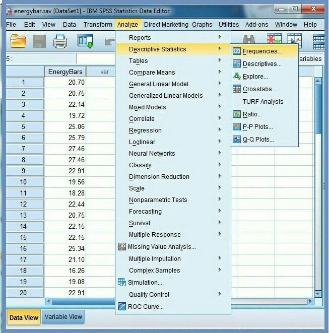
3. Click Analyze, Figure 1
4. Click Descriptive Statistics
5. Click Frequencies…
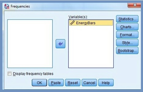
6. Select the test variable (energy bars) in the Frequencies dialog box, Figure 2.
7. Click the arrow button ![]() to move the variable to the test Variable(s) area. Figure 3 displays the test variable that has been moved to the test variable dialog box.
to move the variable to the test Variable(s) area. Figure 3 displays the test variable that has been moved to the test variable dialog box.
8. Click Display frequency tables checkbox to uncheck it.
Our aim is to create a histogram. Therefore, we ignore all other commands and focus on Chart… command.
9. Click Chart… command
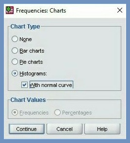
10. Select Histograms option in Frequencies Chart dialog box, Figure 4
11. Check Show normal curve on histogram, Figure 4
12. Click Continue
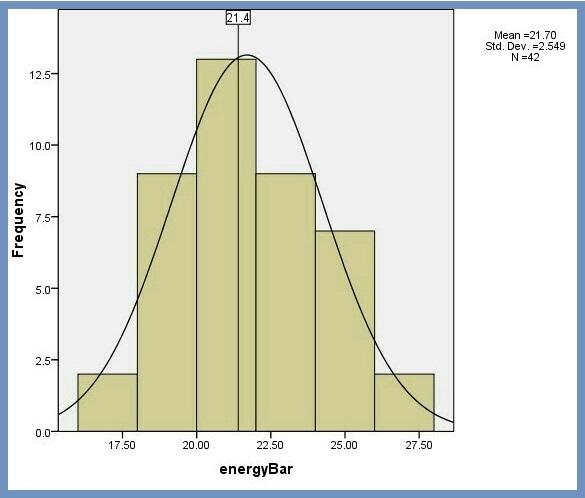
We now have a histogram, Figure 5. By inspection, the histogram shows the data is roughly bell-shaped, and symmetrical, which means they are “even” on both sides of the center. So, our assumption of a normal distribution of the energy bars data seems reasonable.
We’ll revisit this topic as a requirement for normally distributed data for one sample t-test. To learn more about how to carry out normality test for one sample t test, … click here >>>
(b) Normality Test for Independent Samples T Test
Normally distributed data is a requirement for independent samples t-test. These are four methods you can use to test for normality in 2-sample t test:
- Shapiro-Wilk test of normality
- Skewness and Kurtosis
- Histograms
- Normal Q-Q Plots
In this example, we’ll use quantile-quantile plots (Q-Q plots) to investigate whether or not a variable is normally distributed, particularly, with two sample t test. Our dataset is the test scores for 18 students – 10 weekend and 8 regular students.
To create a Q-Q plot, we do the following tasks:
1. Launch SPSS
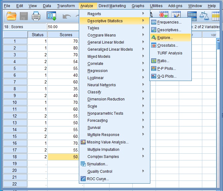
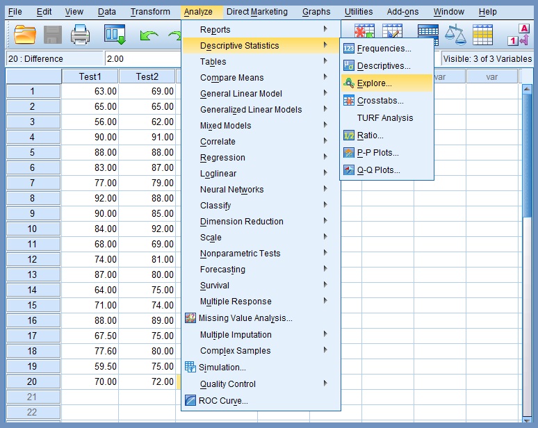
2.Click Analyze, Figure 6
3. Click Descriptive Statistics
4. Click Explore…
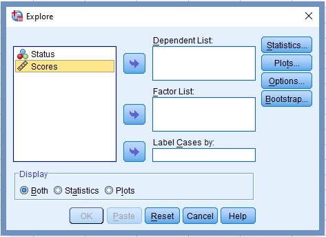
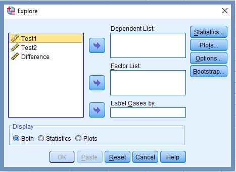
The Explore dialog box opens, Figure 7
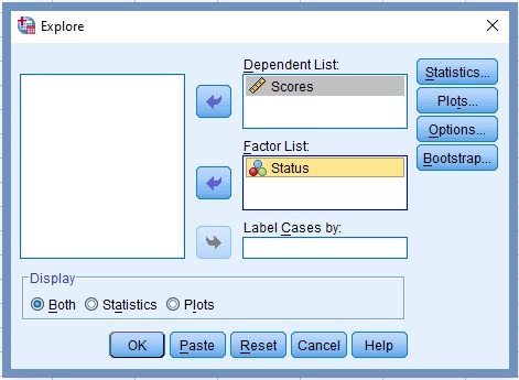
5. Transfer the variable scores into the box labelled Dependent List, Figure 8
6. Click the command labelled Plots…
The Explore-Plot dialog box opens, Figure 9. Make sure the box next to Normality plots with tests is checked.
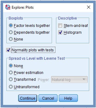
7. Click Continue
8. Click OK
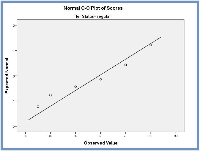
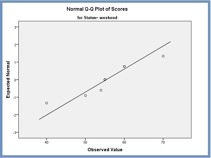
The Output for normal Q-Q plot procedure is displayed in Figures 10 and 11:
Normal Q-Q plot of Scores for regular – control. From the normal Q-Q plots Figure 10 and Figure 11, we note that most of the residuals fall along a roughly straight line at a 45-degree angle. This suggests that the residuals are approximately normally distributed.
Normal Q-Q plot of Scores for weekend – treatment. The normal Q-Q plot for weekend defined as treatment is displayed in Figure 11.
We’ll revisit this topic as a requirement for normal distribution of data for independent samples t-test. To learn more about how to carry out normality test for independent samples t test, … click here >>>
(c) Normality Test for Paired Samples T Test
We can test for normality of paired t test by using the Shapiro-Wilk test of normality since our sample size is small (n<50). We use dataset in Table 2 to illustrate how to check normality for paired samples t test. In this “matched pairs” design, our interest is to establish whether the distribution of the change differences in the dependent variable between the two related groups (test1 and test2) is approximately normally distributed.
| Student | Test1 | Test2 |
| Mercy | 63 | 69 |
| Muna | 65 | 65 |
| Ama | 56 | 62 |
| Kate | 90 | 91 |
| Amama | 88 | 78 |
| John | 83 | 87 |
| Aasim | 77 | 79 |
| Julia | 92 | 88 |
| Jamila | 90 | 85 |
| Zain | 84 | 92 |
| Jean | 68 | 69 |
| Indra | 74 | 81 |
| Susan | 87 | 80 |
| Ruhia | 64 | 75 |
| Miski | 71 | 84 |
| Haneen | 88 | 89 |
We use SPSS procedures to create the change difference variable – difference between test2 and test1. We then use the change difference to determine whether the normality of distribution of our random sample is approximately normally distributed. To learn more about how to use SPSS procedures to build executable expressions that can create a new value from existing values, … click here>>>
To perform Shapiro-Wilk normality test, we do the following tasks:
1. Launch SPSS
2.Click Analyze, Figure 12
3. Click Descriptive Statistics
4. Click Explore…
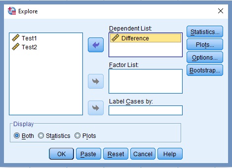
The Explore dialog box opens and displays the original two sample variables (test1 and test2) together with Difference, the new “change” variable Figure 13.
5. Transfer the variable Difference to the Dependent List box, Figure 14.
6. Click the command labelled Plots..
The Explore-Plot dialog box opens, Figure 15. Make sure the box next to Normality plots with tests is checked
7. Unchecked Stem-and-leaf Descriptive option.
8. Check Histogram under Descriptive field.
9. Check Normality plots with tests box.
10. Click Continue
11. Click OK
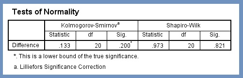
The resultant output has a bunch of outputs tables and plots. However, the only table we’re looking for is Shapiro-Wilk Tests of Normality, Figure 16.
From Figure 16 the Sig. value of the Shapiro-Wilk Test is greater than 0.05, and as a rule of thumb, we fail to reject the null hypothesis since .821 >.05. This suggests that our data set (paired difference) is from a normal distribution.
We revisit this topic as a requirement for normal distribution of data for paired samples t-test. To learn more about how to carry out normality test for dependent samples t test, … click here >>>
Assumption 5: Outliers
There should be no significant outliers. Outliers are simply single data points within a data that do not follow the usual pattern. The problem with outliers is that they can have a negative effect on the t-test, thereby reducing the validity of test analysis.
The simplest way to detect outliers is to draw box plots. Box plots, also known as box and whisker plots, are easy ways to graphically visualize the distribution of the data you’re analyzing. The box demonstrates the central value (50%) of the data, with a line in the middle that shows the median value. The lines extending from the box capture the range of the remaining data. Any data point that falls outside the lines is an outlier, Figure 12.
SPSS uses a circle to mark any outliers. Far outliers, which are more likely to be true outliers, are marked with a star. Next to an outlier icon is a number. The number corresponds to the listed dataset in your Variable View list.
Handling Outliers. When you encounter outliers in your data, there are a few ways to handle them:
Removing outliers. If there is no reasonable scientific basis for an outlier to be in the dataset, one of the easy ways to tackle the issue is to remove the data point. Problematic outliers that represent the following categories should be removed:
- measurement errors
- data entry
- processing errors
- poor sampling
Replacing outliers with closest value to median. If you have just a few data points that are outliers, you could replace them with the next closest value to the median.
Replacing outlier with mean of population. We can tackle outliers by replacing them with the mean of the remaining values without the outlier. The setback for this approach is that we run the risk of distorting the distribution.
Overlooking outliers. Oftentimes, outliers are overlooked by analysts. Some outliers represent natural variations in the population, and they should be overlooked. These are called true outliers. It’s best to remove outliers only when we have a sound reason for doing so.
Assumption 6: Homogeneity of Variances
The assumption of homogeneity of variance is an assumption of the independent samples t-test that all comparison groups have the same variance. We may use any of the following methods to check the homogeneity of variances for 2-sample t test:
Levene’s Test for Variance. We can test this assumption in SPSS Statistics by using Levene’s test for homogeneity of variances. To learn more about how Laverne’s Test is used for independent-sample data … Click here >>
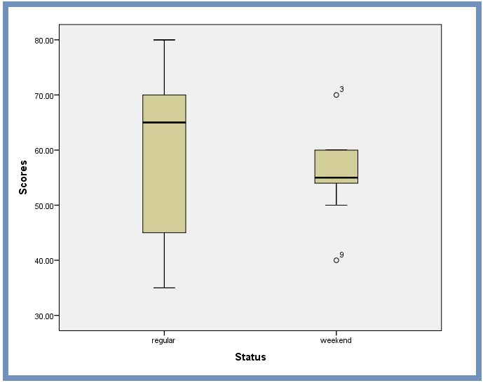
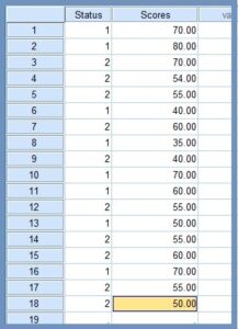
Box Plot for Comparing Variances. We can also use SPSS procedures to look at boxplots to get an idea of what to expect when we conduct independent samples t test. We use the hypothetical data in Figure 13 to compare variances:
To compare the variances of the two groups in the given data, we retrieve the boxplot from the bunch of tables in our previous tutorials on independent t test, see Normality Test for Independent Samples T Test
From Figure 14, we notice that the total length are not about the same for both the two groups. This confirms that the two variances are not equal. Also, from this boxplot, it is clear that the spread of observations for regular is much greater than the spread of observations for weekend. We can safely estimate that the variances for these two groups are quite different.
Welch’s Test for Unequal Variance. We use Welch’s test to compare the means of two independent groups when sample sizes and variances are unequal between groups
In practice, when we compare the means of two groups it is unlikely that the standard deviations for each group will be identical. This makes it a good idea to just always use Welch’s t-test, so that we don’t have to make any assumptions about equal variances.
To learn more about Welch’s test for unequal variance watch the video (Figure 14)
Figure 14: Welch’s test for unequal variances
To learn more about how to carry out homogeneity test for independent t test, ….Click here>>>
Citation Information
If you want to cite this lesson, you may use the following APA information:
- Author: Mahama, A.
- Date of publication: Use the 2024, February 18 or the last date the lesson was modified.
- Title: Data requirements for t test
- URL of lesson: https://thecalleacademy.thecallinfo.com/lessons/data-requirements-for-t-tests/
- xxx is the date you retrieved the lesson from the online source
Example
Mahama, A. (2024, February 18). Data requirements for t test. Retrieve xxx from https://thecalleacademy.thecallinfo.com/lessons/data-requirements-for-t-tests/
References
Amanda, S. (2023). STM1001 Topic 6: t-tests for two-sample hypothesis testing. Retrieved January 12, 2024 from https://bookdown.org/content/f9d035ed-86ea-4779-ad01-31acc973f0dd/
Lund. (n.d.). Testing for normality using SPSS statistics. Retrieved August 31, 2023 from https://statistics.laerd.com/spss-tutorials/testing-for-normality-using-spss-statistics.php
Khan, M. (April 8, 2022). How to detect outliers. Retrieved September 12, 2023 from https://godatadrive.com/blog/how-to-detect-outliers
Stephanie G. (2023). Outliers SPSS – from StatisticsHowTo.com: Elementary Statistics for the rest of us! Retrieved September 11, 2023 from https://www.statisticshowto.com/outliers-spss/
▣▣▣
