
Testing assumptions of independent-samples t–test
Introduction
In teaching the assumptions for an independent-samples t-test, it’s essential to emphasize that this statistical test compares the means of two distinct groups to determine if there is a statistically significant difference between them. Before conducting the test, we must ensure that certain assumptions are met, as these validate the accuracy and reliability of the results.
Understanding and verifying these assumptions allows for meaningful application of the independent-samples t-test, ensuring that any detected differences are due to the groups themselves rather than unmet statistical conditions.
This test is sometimes referred to as:
- Independent t-test
- Independent-measures t-test
- Independent two-sample t-test
- Student t-test
- Two-Sample t-test
- Uncorrelated scores t-test
- Unpaired t-test
- Unrelated t-test
Learning Outcomes
By the time you complete this lesson, you should be able to:
- verify the assumptions for independent t-test forsample data
- Shapiro-Wilk test of normality
- carry out Welche’s test for unequal variances
- Homogeneity of Variances
Problem Statement
The hypothetical study evaluates the effect of PowerPoint on test scores of students. The sample for the study comprises 18 students randomly assigned to two groups – treatment and control:
- 8 weekend students by treatment – receiving instructions with PowerPoint intervention
- 10 regular students by control – receiving instructions with no PowerPoint intervention
The performance of the 18 students at the end of the training is expressed as Scores. For Status, the numbers 1 and 2 represent PowerPoint instructions and no PowerPoint instructions respectively. The SPSS data view of the sample data is shown in Figure 1.

Data Requirements for Independent T Test
Before we carry out the independent t test, we need to check the integrity of our sample data. We do this by examining the different assumptions that our sample dataset must satisfy for the t-test results to remain valid.
Assumption 1: Continuous Scale of Data
The given test scores (the dependent variable) from the problem statement are measured on a continuous scale: 70.00, 30.00, 55.00, etc., Figure 1.
Assumption 2: Data Type
The independent variable (status) consists of two categorical, independent groups – weekend (PowerPoint intervention) and regular (no PowerPoint intervention).
Assumption 3: Relationship of Groups
There is no relationship between a weekend student who receives instructions with aid of PowerPoint, and a regular student who does not receive instructions with PowerPoint intervention.
Assumption 4: Randomness of Data
The narration from the problem statement indicates the 18 students for the study are randomly selected.
Assumption 5: Normality of Data
In SPSS Statistics, we can test for normality by using Shapiro-Wilk test, Skewness and Kurtosis, Histograms, and Normal Q-Q Plots.
In this example, we’ll use Shapiro-Wilk test and normal Q-Q plot to determine whether or not our sample data is normally distributed by doing the following tasks:
1. Launch SPSS
2.Click Analyze, Figure 2
3. Click Descriptive Statistics
4. Click Explore…
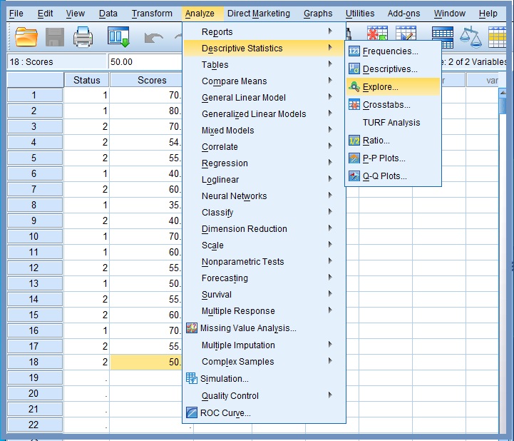
The Explore dialog box opens, Figure 3.
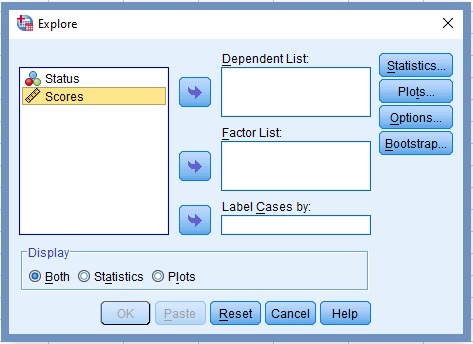
5. Transfer the scores variable to the box labelled Dependent List, Figure 4
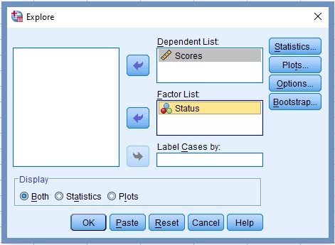
6. Click the command labelled Plots…
The Explore-Plot dialog box opens, Figure 5. Make sure only the boxes next to Normality plots with tests and Histogram are checked.
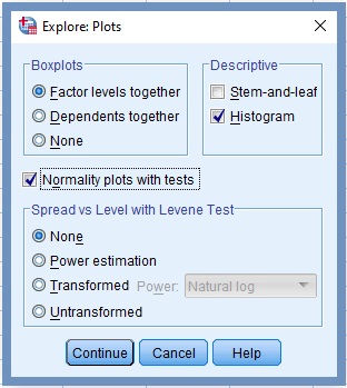
7. Click Continue
8. Click OK
Output of Normality Test
The SPSS procedures create a bunch of outputs. However, the only plots and table of interest to us are: normal Q-Q plots, box plot, and Shapiro-Wilk test.
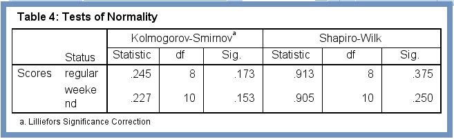
Shapiro-Wilk Test of Normality. Since our sample size is less than 50, it’s more appropriate to use the Shapiro-Wilk test as a numerical means of determining normality of the dependent variable.
From Figure 6 the Sig. values (.375 and .250) of the Shapiro-Wilk test are greater than 0.05. We can safely assume the dependent variable is approximately normally distributed for the independent variable groups.
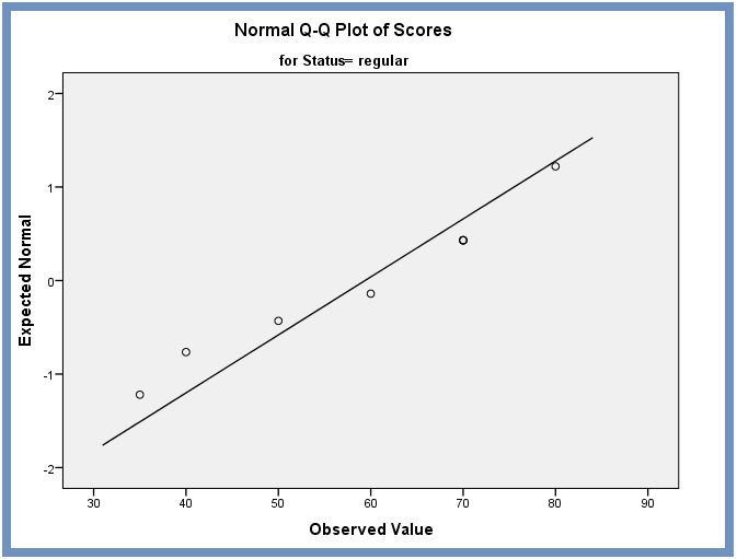
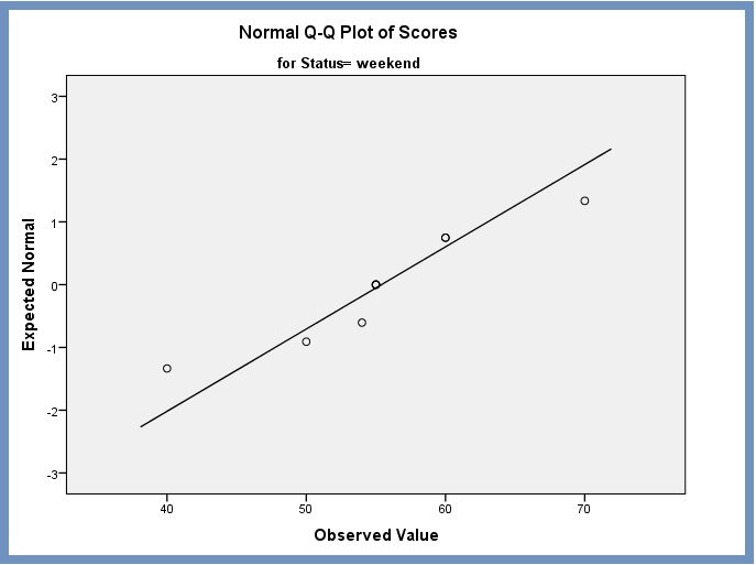
Normal Q-Q Plots. The plots give us a graphical visualization and assessment of normality. In the Q-Q plots (Figure 7 and Figure 8), most of the residuals fall along a roughly straight line at a 45-degree angle. This suggests that the residuals are roughly normally distributed.
Note
Assumption 6: No Outliers
There should be no significant outliers. Outliers are simply single data points within a dataset that do not follow the usual pattern. Their presence in a dataset can reduce the validity of t test results.
Outliers represent natural variations in the population, and can be overlooked. Other outliers may result from incorrect data entry, equipment malfunctions, or other measurement errors. They are deemed problematic and should be removed.
Striking off outliers is usually a judgment call. In our sample, we chose not to delete outliers since the dataset is a collection of fictitious data meant to demonstrate the concept of 2-sample t-test.
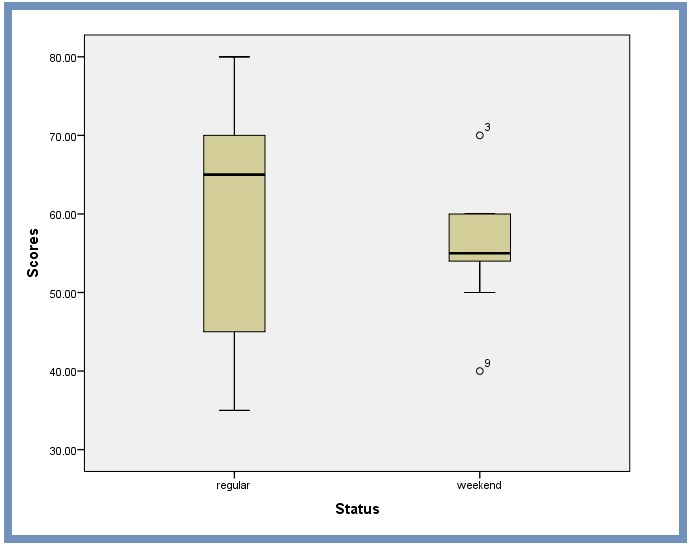
We can use the box plot in Figure 9 to detect if any outliers exists in our dataset. The box plot demonstrates the central value (50%) of the data, with a line in the middle that shows the median value. The lines extending from the box capture the range of the remaining data.
Any data point that falls outside the lines indicates an outlier. SPSS uses a circle (°) or a Star (*) to mark any outliers. The number next to an outlier icon corresponds to the listed item in the dataset. This corresponds to the third (70.00) and ninth (40.00) of our dataset, see Figure 1.
Note
Assumption 6: Homogeneity of Variances
The assumption of homogeneity of variance is an assumption that all comparison groups of the independent samples t-test have the same variance. We will use the Box plot to gain insight into the homogeneity of variances for our 2-sample t test.
Box plot for comparing variances. One of the plots in the previous output (Figure 9) is a comparative box plot. The graphical visualization gives us a clue on variances for these two groups of the sample.
The total length (spread of observations) are not about the same for both the two groups, Figure 9. This confirms that the two variances are not equal. However, from this boxplot, it is clear that the spread of observations for non use of PowerPoint (Regular) is much greater than the spread of observations for use of PowerPoint (Weekend). We therefore can safely estimate that the variances for these two groups are quite different.
Welch’s test for unequal variance. We can go beyond the boxplot and consider Welch’s test, a numerical means of comparing variance of groups so that we don’t have to make any assumptions about equal variances.
To learn more about Welch’s test for unequal variance watch the video (Figure 10):
Figure 10: Welch’s test for unequal variances. Credit: Statology.org
Our focus at this stage is to use Welch’s test to compare the means of two independent groups because of our small sample sizes and also, the variances are unequal between groups. We perform Welch’s test by doing the following tasks:
1. Launch SPSS
2. Click Analyze, Figure 11
3. Click Compare Means
4. Click One-Way ANOVA…
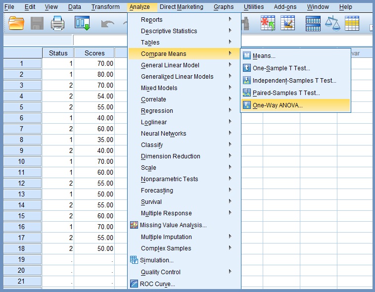
The One-Way ANOVA dialog box displays two variables of 2-samples t test, Figure 12.
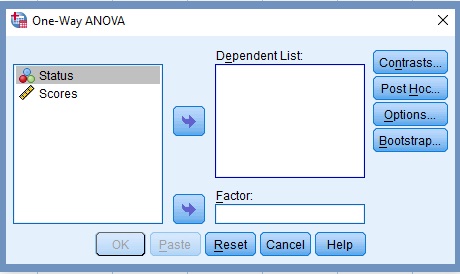
5. Transfer Scores to the Dependent List pane,Figure 13
6. Transfer Status to the Factor textbox
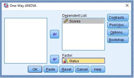
7. Click Options … command, Figure 13
8. Click BBorown-Forsythe checkbox in the One-Way ANOVA: Options dialog box, Figure 14
9. Click Welch checkbox in the One-Way ANOVA: Options dialog box, Figure 14
10. Click Continue command
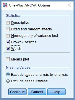
11. Click OK
The resultant output is displayed in Figure 15. Our interest at this stage is Robust Tests of Equality of Means. It displays Welch’s Sig. value of .536.
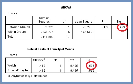
For unequal variance, the null hypothesis can be stated as: the two population means are the same but the two population variances may differ. For our Welch’s test, we reject the null hypothesis if Sig is less than the level of significance. From Figure 15 we cannot reject the null hypothesis since the Sig value is greater than the level of significance (i.e., .535>.05). This suggests that a relationship does exist between our set of variables and the effect is statistically significant.
Citation Information
If you want to cite this lesson, you may use the following APA information:
- Author: Mahama, A.
- Date of publication: Use the 2023, February 27 or the last date the lesson was modified.
- Title: Conducting independent sample t test
- URL of lesson: https://thecalleacademy.thecallinfo.com/courses/research/data-analysis-1/lessons/conducting-independent-samples-t-test/
- xxx is the date thus lesson is retrieved
Example
Mahama, A. (2023, August 26). Conducting one sample t test. Retrieve xxx from https://thecalleacademy.thecallinfo.com/courses/research/data-analysis-1/lessons/conducting-independent-samples-t-test/
References
Daniel, T. (202017, December 10). https://youtu.be/-qGFZFOQx7Q [Video]. Retrieved August 18, 2023 from YouTube: https://youtu.be/vII22ZnFOP0
Editorial Director. (2023). How should p values be reported? Retrieved June 02, 2023 from
https://support.jmir.org/hc/en-us/articles/360000002012-How-should-P-values-be-reported-
Kent State University. (2021). Paired samples t test. Retrieved February 11, 2023 from https://libguides.library.kent.edu/spss/pairedsamplesttest
Lund Research Ltd. (2018). Dependent t-test using SPSS statistics. Retrieved July 15, 2023 from
https://statistics.laerd.com/spss-tutorials/dependent-t-test-using-spss-statistics.php
Zach, B. (May 29, 2019). Welch’s t-test: When to use it + examples. Retrieved September 10, 2023 from http://www.statology.org/welchs-t-test/
▣▣▣
